By Ami Levin, SQL Server MVP
SQL Server implements three different physical operators to perform joins. In this article series we will examine how each operators works, its advantages and challenges. We will try to understand the logic behind the optimizer's decisions on which operator to use for various joins using (semi) real life examples and how to avoid common pitfalls.
I'm sure you are all very familiar with T-SQL joins so I'll skip the introductory part this time. For this article, I'll focus on the most common type of join, the 'E-I-J' (or 'Equi-Inner-Join') which is just a cool sounding name for an inner join that uses only equality predicates for the join conditions. With sadness, I will skip some extremely interesting issues concerning joins such as logical processing order of outer joins, NULL value issues, join parallelism and others. This article focuses on helping you make your E-I-J joins faster. We'll accomplish this by helping you understand how the SQL Server optimizer decides which physical operators it will use to carry out your query joins. We'll show you situations where the SQL Server optimizer is occasionally tricked into choosing a slower method by the characteristics of the data and SQL you wrote. If you understand these pitfalls, you can code to overcome them, thus speeding up your queries - and impressing your colleagues and bosses.
As amazing as the SQL Server optimizer can sometimes be, it's not making its decisions intuitively. It's using the information it has to work with. Recall that a join is basically 'looking for matching rows' from two inputs, based on the join condition. The creators of the optimizer have made three techniques available to it for carrying out these joins:
- Nested Loops
- Merge
- Hash Match
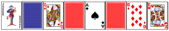
For this article series I will use an analogy of two sets of standard playing cards. One set with a blue back and another with a red back that need to be 'joined' together according to various join conditions. The two sets of cards simply represent the rows from the two joined tables, the red input and the blue input - "Now Neo - which input do you choose"?
Nested Loops
Probably the simplest and most obvious operator is the nested loops operator. The algorithm for this operator is as follows:
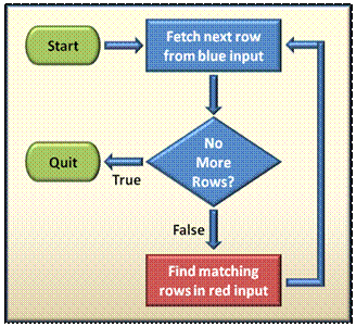
Flowchart 1 - Nested Loops
The 'outer loop' consists of going through all rows from the blue input and for each row; some mysterious 'inner operator' is performed to find the matching rows from the red input. If we would use this operator to join our sets of cards, we would browse through all the blue-back cards and for each one we would have to go through all the red-back cards to find its matches. Not the most efficient way of matching cards but it probably would be most people's first choice... if there are only a handful of cards to match.
Let's take a closer look and see when nested loops are a good choice. The first parameter to consider, as with any iterative loop, is the number of required iterations. For nested loops to be efficient, it requires at least one relatively small row set to be used as the outer loop input that determines the number of iterations. Remember that this does not necessarily reflect the number of rows in the table but the number of rows that satisfy the query filters.
The second parameter to consider is the (intentionally) vague "Find matching rows in red input" part in Flow Chart 1 above. Assuming that we do have a small input for the outer loop, hence a small number of required iterations, we now must consider how much work is required to actually find the matching rows in every iteration. "Find matching rows" might consist of a highly efficient index seek but it might require a full table scan if the join columns are not properly indexed; making nested loops a far less optimal plan. Since it is very common for joins to be performed on one-to-many relationships, and since the parent node in these relationships is often the smaller input (the 'one' in the 'one-to-many'), and since this parent node is always indexed (must be a primary key or a unique constraint), the well known best practice rule that requires that FK columns should be indexed, now makes perfect sense, doesn't it?
Let's see a few examples:
* Note: All the queries used in this article can be found in the demo code file, plus a few more. I highly recommend that you play around with the code, change parameters and select list columns, try to use outer joins and even create some indexes and see how they affect the query plans. Just remember to drop your indexes before proceeding to the next query so that the demo plans will remain valid.
Small outer loop with a well indexed inner input
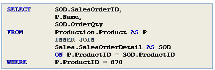
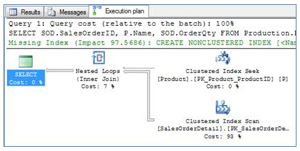
The most obvious case for nested loops is when one input is very small (is 1 row small enough?) and the other input is ideally indexed for the join. In Execution Plan 1 you can see that the optimizer retrieved the single row for product 870 from the Product table using a PK clus
tered index seek (needed to retrieve theProduct Name) and all the matching Order IDs were retrieved using the non clustered index on the Product IDcolumn of the Order Detail table.
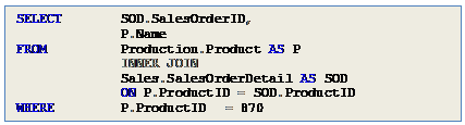
Query 1
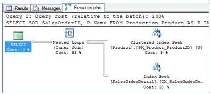
Execution Plan 1
* Tip: The optimizer was clever enough to duplicate the filter for Product ID to both tables although the predicate specifies only the Product table. Since the filter and the join condition are based on the same column and since the join is an equi-join, the optimizer knows that when constructing its physical operators, it can add a second predicate ‘AND SOD.ProductID = 870’ to optimize the data access for the Order Detail table.
Nested loop joins with table scans
If we just add the Order Quantity column to the select list as in Query 2 , the index on Product ID (which does not contain the Order Quantity column) is now not enough to 'cover' the query, meaning that it does not include all the data required to satisfy the query. The optimizer can either perform a 'lookup' (Use the pointer from the index to fetch the full row from the table itself) for each Order Detail row to get it (nearly 5,000 lookups...) or alternatively it can simply scan the Order Detail table, retrieve both Product ID and Order Quantity. In this case, since there is just one Product row to join hence the table only needs to be scanned once, and since the table is not very large (which would make the scan expensive), the single scan option is probably better than the alternative of performing thousands of lookups. Indeed, this is exactly what the optimizer chooses to do in this situation as you can see in Execution Plan 2.
Query 2
Execution Plan 2
* Exercise: Try to change the predicate to ‘P.ProductID IN (870,871)’. This would mean that now, to use the same plan as above will require two full scans instead of just one. Do you think that this will still be the most efficient plan? Try it and see what plan the optimizer chooses. You can find the code for this exercise (Code sample #2b) in the demo code.
Nested loop joins with lookups
Now, let's play around a bit with the parameters. In Query 3, I have changed the predicate to filter for three products instead of one, but I used products that are far less commonly ordered. Think of three colors of 'White-Out' ('Tipp-Ex' for you Europeans) for the computer screen - not the hottest seller... Now, a slightly different use of nested loops emerges. Note that product 870 exists in nearly 5,000 Order Detailrows, but only 13 Order Detail rows contain one or more of Query 3's three products (897,942,943). The optimizer always consults the column statistical histograms so it is very aware of this fact. To join only product 870, the optimizer chose to perform a single scan instead of an index seek + 5,000 additional lookups. For the three products in Query 3, it could either perform three full scans or revert to using an index seek + 13 additional lookups. What do you think is the right choice?
The answer is graphically portrayed in Execution Plan 3 . Note that the execution plan incorporates two nested loop physical operators, and that both constitute logical inner joins. The one on the right is our actual table join, and the one on the left denotes the full-record lookup from the Order Detail table (required in order to retrieve the Order Quantity) which, in a sense, is also a join between the Order Detail table and the result of the first join.
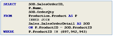
Query 3
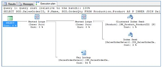
Execution Plan 3

One of the most common pitfalls of the query optimizer is under-estimating the number of required iterations for a nested loops operator due to (partial list):
- Statistical deviations
- Outdated statistical data
- 'Hard to estimate' predicates such as compound expressions, sub queries, functions or type conversions on filter columns
- Multiple predicates estimation errors
When analyzing a poorly performing query, one of the first things I do is to look at the 'Estimated number of rows' vs. the 'Actual number of rows' figures of the outer input of the nested loop operator. The outer input is the top one in the graphical query execution plan. See for example Execution Plan 4 . I've seen many cases where the optimizer estimated that only a few dozen iterations will be required, making nested loops operator a very good choice for the join, but in fact tens (or even hundreds) of thousands of rows satisfied the filters, causing the query to perform very badly.
For Query 4 below, the optimizer estimated that ~1.3 products will satisfy the query filters when in fact, 44 products did. This seemingly small error led the optimizer to believe that only 616 rows will be matched from the Order Detail table and that estimation made it choose the same plan as the previous example, using an index seek and additional lookups. The optimizer estimated that it will require only 616 key lookups when in fact, 20,574 were required. This might seem at first like a flaw in the optimizer, but only to the degree that mind reading is hard to program. You'll see why in the answer to Challenge #1 at the end of this section.
* Challenge #1: Can you guess what misled the optimizer to make the estimation error? See the answer at the end of this section.
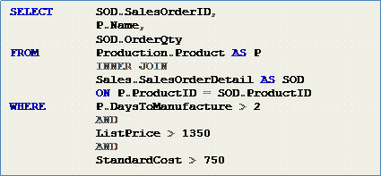
Query 4
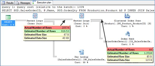
Execution Plan 4
* Exercise: The demo code contains Query 4 as shown here, plus hints that force the optimizer to use nested loops, hash match or merge joins respectively (Queries 4b, 4c and 4d). Use the demo code to execute these query variations. Trace the executions with profiler to benchmark these alternatives and see if the optimizer was correct to prefer nested loops for this query. Remember that logical reads might be misleading so pay close attention to both CPU and duration when evaluating the queries’ true efficiency.
Wicked a-sequential page cache flushes
One more issue we need to consider with nested loops is the issue of sequential vs. a-sequential page access patterns. You might recall from myprevious article that nested loops are characterized with a high number of logical reads, as the same data page might be accessed multiple times. For small row sets, this is usually not an issue as the pages are cached once and subsequent reads are performed in memory. But, if the system experiences memory pressure and in the common case where the outer loop consists of a large number of rows where the distribution of the data (in respect to the order of the join columns retrieved for the outer loop) within the pages is more or less random, a real performance nightmare might occur when a page is repeatedly flushed from the buffer cache only to be physically retrieved a few seconds later for retrieval of another row, for the same join! If you were the query optimizer - go with the flow for a moment - how would you avoid such a performance 'nightmare'?
Feel free to discuss your ideas for potential solutions in the comments section.
* Challenge #1 answer: The filter consists of three predicates. If you inspected each predicate by itself (armed with the statistical distribution histograms of the values in each column), you would see that the predicates are highly selective, meaning that they filter out a large percentage of the rows as the values used are very close to the maximum values for each of the columns. Using AND logical operators for these three highly selective predicates leads the optimizer to estimate that only a few rows will satisfy all three predicates. This is correct from a statistical perspective under the assumption that there is no correlation between the predicates. But... unbeknownst to the optimizer, the values in these three predicates are actually closely related. The query filters for the products that take the longest to manufacture, making them the products with the highest cost, and naturally the ones with the highest list price. So it's more or less the same group of products that satisfy each predicate. These and other conditions which make selectivity extremely hard to estimate are much more common in production systems than most people would think.
I want to use this opportunity to congratulate the Microsoft SQL Server optimizer team for producing an unbelievably intelligent optimization engine which is (IMHO) by far the best of its kind on the market, and it just keeps getting better with every new version. It is getting harder and harder for me to come up with such examples where I manage to make it err.
If you are interested to dive deeper and learn more on joins and their implementation in SQL Server, I highly recommend Craig Freedman's SQL Server Blog on MSDN. Craig has published a series of excellent, in depth articles regarding many more aspects and types of joins.
Part II of this article series will examine the Merge Operator, and part III will discuss the Hash Operator.