By Ami Levin, SQL Server MVP
In this series of short articles, we lift the hood of the SQL Server Optimizer to examine a few of the many clever tricks used to optimize query performance. You'll see that the Optimizer does not limit itself to using only the instructions provided by the written query syntax, but can correctly deduce a more efficient approach from information it gleans from the schema, the query and data statistical information
In Part I, we look at partial aggregate operators - an extremely clever way of downsizing certain large joins into much smaller (and faster) joins.
In my previous series of articles, we examined the three different physical join operators (Nested Loops, Merge and Hash Match) and saw how the Optimizer chooses which is best to use for different types of queries and for varying data patterns. In this series, we will take things one step further and describe some of the other tricks the Optimizer has stored up its sleeve for us when it comes to optimizing query performance. The first sleight-of-hand, known as partial aggregation, is a technique commonly used for joins with particular characteristics. An example follows.
Note : To execute this article's demo code you will need to download the AdvertureWorks2008R2 database from CodePlex. However, this article is written to be a full explanation without using the sample database or code.
Consider the following query:
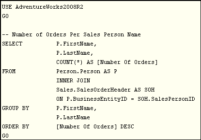
The query itself is quite simple and straightforward. It produces a list of names of sales people and their order counts, arranged so that the highest-producing sales person name is listed first.
It joins the Person table with the SalesOrderHeader table, groups the result by the sales people's first name and last name, and counts the number of orders each sales person has obtained. Note that there is a potential logical issue with this query as grouping by first name and last name does not guarantee uniqueness of sales person because two sales people may share the same name. This may lead to potentially confusing results when "John Smith" is only listed once in the result set, and "his/hers" sales look much larger than either of them expected. But because the AdventureWorksdatabase does not contain identical first and last names, we'll ignore this issue for now.
At first glance, we might expect the Optimizer to take a straightforward approach to execute this simple query:
1. Join the two tables.
2. Group by the first name and last name columns.
3. Count the number of orders in each group.
Obvious enough, isn't it?
Well, let's take a look at the actual execution plan that was used, in the figure below.
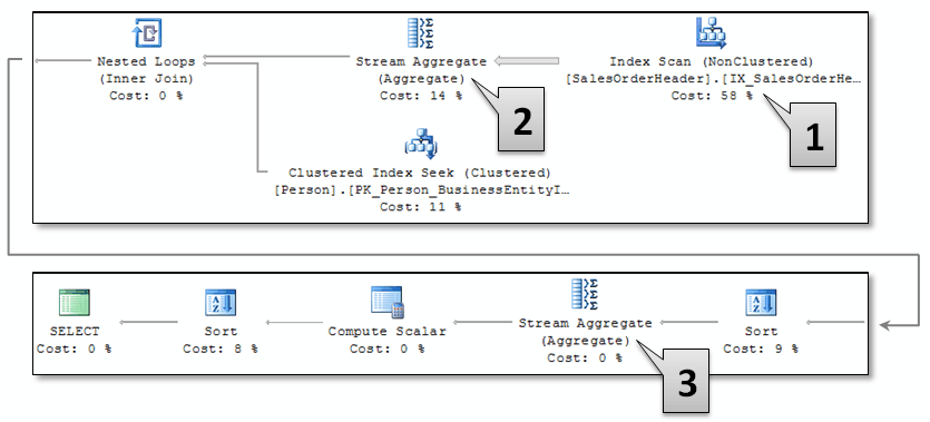
Figure 1 - Actual Execution Plan
The execution plan seems to be exactly as expected, except for the Stream Aggregate operator [2] which follows the Index Scanoperator [1] on the SalesOrderHeader Table. What is it doing there? It can't aggregate order counts by First Name and Last Name quite yet... the First Name and Last Name won't be available until after the join is complete, because those columns are from the Person table which has not been accessed yet... What the heck is going on?
When viewing the Execution Plan in SSMS, you can reveal the following details about this stream aggregate operator by hovering your mouse over its icon:
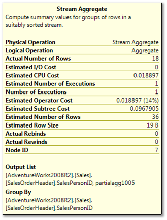
Figure 2 - Properties of Stream Aggregate operator [2]
Look at the Group By section at the bottom. It indicates a grouping of the output by SalesPersonID!? This seems to contradict the query's explicit instruction to group by First and Last Name. Now look at Output List section just above it. Ah... there is a hint... The Output list, a list of SalesPersonIDs, is only a partial aggregate ("Partialagg1005"). So the Optimizer knows that the aggregation (group by) task is not yet complete.
What is it up to?
Let's step into the Optimizer's shoes for a minute. It does not possess human logic. Rather, it works with the facts available to it, and deduces its best approach.
What facts is it working with?
- There are only a handful of sales persons that made orders. 17 to be precise.
Note: The count of sales people is available from the distribution statistics on the SalesPersonID column.To confirm this count for yourself, run the following query:
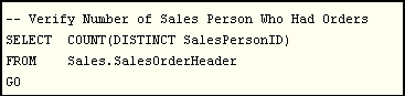
* Teaser: If you look at the 'Estimated Number of Rows'. you will see that the Optimizer estimates that 36 rows will be returned when in fact only 18 were returned. Do you think this is a reasonable estimation error? Can you guess why such errors happen and perhaps how to avoid them?
* Quiz: Why does the 'Actual Number of Rows' indicate 18 rows when we know for a fact that there are only 17 sales person that performed orders? Where did we 'lose' a sales person?
- The query requires only the count of the orders per sales person name, and no data about individual orders.
- There is an index on SalesPersonID.
- There are 31,465 orders made by these 17 people.
- The SalesPersonID is being joined to the BusinessEntityID using an equity predicate.
- The BusinessEntityID is the primary key of the Person table.
From these last two points, the Optimizer can safely conclude that grouping by SalesPersonID will create a super-set of any other potential grouping that will be performed on any columns from the Person table.
Now things are getting clearer.
If the SQL Server Optimizer were to follow the simplest approach, as detailed in the 'expected steps' list above, it would have joined all of the 31,465 rows from the SalesOrderHeader table with the Person table. But it was smart enough to recognize an opportunity to perform a colossal shortcut, and it seized it.
Pre-grouping by SalesPersonID (the Partial Aggregate) enabled the Optimizer to join only 17 output-rows from the scan on SalesOrderheader table instead of all 31,465 rows. It already had the order count for each sales person, which it easily obtained by performing an ordered scan on the SalesPersonID index. This low row count also made the nested loops operator the clear winner in the contest for best join operator, as only 17 index-seek iterations were required for the join - a huge time saver.
After the join was performed, the only remaining task was to sort and group these 17 group rows again. A child's play. The second grouping had to be performed in case there were two different sales people (each with his/her unique SalesPersonID) who had the same first and last names. This would have (perhaps undesirably) summed together the order counts for the company's two men named "John Smith", and perhaps for the first time made "his" sales figures top the charts.
The second grouping (aggregation) is clearly detailed in the properties of the second Stream Aggregate operator [3] we saw in the Actual Execution Plan (Figure ).
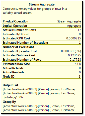
Figure 3 - Properties of Stream Aggregate operator [3]
In the Output List section of this details box, you can see the reference to a global aggregate operation ("globalagg1006"). This indicates that the Optimizer is performing the final Group By action - that is, by the First Name and Last Name columns requested in the original query. The relationship between the partial aggregate and the global aggregate can be seen in the 'Defined Values' row in the properties window of the stream aggregateoperator:
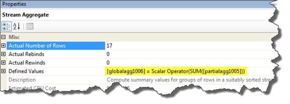
Figure 4 - Full Properties Window of Stream Aggregate operator [3]
The order counts of each sales person ID are summed up into the new (sub) groups, by the sales person names. In our example, the two groups happen to be identical.
* Tip: Opening the properties window: In the graphical execution plan pane of the query window in SSMS, click to select the left 'stream aggregate' operator (3) and then press F4 to open its fully detailed properties window.
Makes you wonder just how much smarter the SQL Optimizer can be? That will be explored in the second part of the "Under the Hood" series, when we'll see even more delicious treats from the kitchen of the SQL Server query Optimizer team.